
Ch. 2: Motion in a Straight Line
Reading
College Physics, Ch. 2
AP Classroom: Unit 1 "Kinematics" (continued)
AP Princeton Review: Ch. 4
Topics
Labs
College Physics, Ch. 2
AP Classroom: Unit 1 "Kinematics" (continued)
AP Princeton Review: Ch. 4
Topics
- Displacement, speed, velocity, and acceleration
- The "Big Five" equations of motion
Labs
- Galileo's Inclined Plane lab. Instructions below. Remember to bring the lab handout to class!
- Skate Park weblab. Instructions below.
Homework
Homework is hosted in Canvas. Other handouts/videos below...
Homework is hosted in Canvas. Other handouts/videos below...
| 1._Velocity problems_Canvas MCQ's WORKED 2023.docx |
| 1._Acceleration_problems_to use with Canvas ALSO SEE VIDEO__2023_.docx |
Lecture outline:
Velocity
vavg = (x2 – x1) / (t2 – t1)
Acceleration
aavg = (v2 – v1) / (t2 – t1)
Velocity
- Velocity indicates how your location changes with time. It is distance divided by time, as in “miles per hour” or “meters per second”
- We write the formula as follows:
vavg = (x2 – x1) / (t2 – t1)
Acceleration
- Acceleration indicates how your velocity changes with time.
- Positive acceleration means "speeding up". Negative acceleration (i.e. deceleration) means "slowing down".
- We use units of "meters per second per second" or "meters per second squared".
- We write the formula as follows
aavg = (v2 – v1) / (t2 – t1)
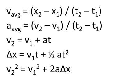
The five (5) equations of motion: "The Big Five"
- You will use these 5 equations for the next several chapters! Locate them in your book and mark the page; you will be referring to them over and over again.
Lecture video
This vid is important and covers the "typical" types of velocity-acceleration problems
This vid is important and covers the "typical" types of velocity-acceleration problems
Galileo's Inclined Plane lab
REMEMBER TO BRING THE LAB HANDOUT!
Galileo Lab, part 1
Galileo Lab, part 2
REMEMBER TO BRING THE LAB HANDOUT!
- In this lab exercise we reproduce Galileo's famous inclined-plane experiment using a modern Vernier cart and track set at 3 different angles.
- This is exactly what Galileo did using a bronze ball and wooden track with a groove down the middle. Galileo, however, didn't have a movie camera with an electronic timer; his "clock" was allowing water to drip into a container and then weighing the container!
- Our goal is to estimate 'g', the acceleration due to gravity on planet Earth, and compare with the known value of 9.8 m/sec^2.
Galileo Lab, part 1
- Elevate one end of the track at 3 different heights, such that you have a 'slow', 'medium', and 'fast' cart moving down the track.
- Using a movie camera (or motion app) and cart, record "distance vs. time" down the 2-meter track for each scenario: 1) slow, 2) medium, 3) fast. Record the raw data in the form of a table. See example below.
- Create a "distance-vs-time plot" of the raw data we gathered. You will have 3 curves, one for each ramp angle we used. See example below.
- Label everything and make it look nice & professional. Use circles, squares, and triangles as shown. Sketch nice-looking best-fit curves. TAKE PRIDE IN YOUR WORK.
Galileo Lab, part 2
- Compute the final velocity of the cart for each track-scenario: Do this by carefully drawing a tangent line (at a convenient spot near the top of each curve), constructing a triangle, and calculating the slope of the curve at that point. Recall that slope is equal to (y2-y1)/(x2-x1), which is the same as "rise-over-run". If you draw your triangle carefully, you can fairly-easily count-out (y2-y1)/(x2-x1) on your graph paper, which will give you the slope at that point, which is equivalent to 'velocity' in m/s. Again, recall that when you plot "distance-vs-time", with distance on the Y-axis, the slope of the curve at any point is equal to 'velocity'. The velocity you are calculating is the 'final velocity' of the cart - or at least the final velocity at the 'time' you draw your tangent line at. See example below.
- Use equation #5 of the Big Five (listed above) to compute the acceleration of the cart down each track: 1) slow track, 2) medium track, and 3) fast track.
- Using the principle of "similar triangles", calculate the acceleration of gravity 'g' for each of the 3 runs. See example below.
- Analysis: compare your 3 values of 'g' with the known value of 9.8 m/s^2. Compute the % error between your average value and the 'true' value of 9.8 m/s^2. Try to explain any differences.
| galileo_lab__part_1_lab handout_-_graphs_and_raw_data_table |
| galileo_lab__part_2_lab handout_-_final_lab_report |
Use this graph paper: http://www.printfreegraphpaper.com/gp/e-i-110.pdf
"Skate Park" weblab
Follow the instructions in the handout below. Upload your completed work to Canvas by the due date.
Online Curve Fitting Calculator: elsenaju.eu/Calculator/online-curve-fit.htm
Follow the instructions in the handout below. Upload your completed work to Canvas by the due date.
Online Curve Fitting Calculator: elsenaju.eu/Calculator/online-curve-fit.htm
| 1._skate_park_weblab__rev_2023_.docx |